General Kinematics
General kinematics is based around the description of the motion of objects - disregarding the forces acting on them, such as motors. This section will concentrate on the kinematics models, and saving the driving forces for another tutorial. Planning and modeling the kinematics for a system allows for simulation and testing of both simple and complex projects without picking up a single hardware tool. With advanced robot and motion controllers becoming more common-place and accessible by the day, a near-universal robotic controlling system can be a boon for hobbyists and advanced users alike. Kinematic position and velocity models as well as the back-end controllers work to drive the mechanism or simulation quickly and accurately.
Forward Kinematics
Kinematic models are generally split into two halfs: Forward and Inverse. Forward Kinematic models are used to determine the position and orientation of the robot end effector in terms of the joint link lengths and angles. The basic robot limb can be an arm with a gripper/manipulator, a leg with a foot or even a wheel. Link lengths, offsets and angles, when analyzed, give one possible stance in 3D space (assuming rigid or semi-rigid hardware); this means it can be absolutely and directly solved for.
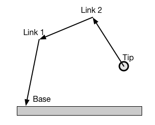
In standard forward kinematic models there’s no need for iterative solvers, unlike some Inverse Kinematics, which will be covered in the next section. The figure below shows the order of analysis, starting at the base and flowing through the links until the endpoint is reached. The characteristics of the link angles and lengths are used to calculate the equations of motion from the base to the tool tip.
Inverse Kinematics
The Inverse Kinematics model is used to determine the required joint angles or conditions of the robotic arm in order to place the end effector at a desired position and orientation in 3D space. Deriving the inverse kinematics of a system are typically much more difficult than computing the forward kinematics. For simple examples, it can be directly solved using a number of analytic approaches, assuming the Degrees of Freedom (DOF) of the end effector equals the DOF of the system. For example, a 2 link/DOF robot arm can only place its end effector in 2 DOF, within the combined reachable range of both of the limbs, attempting to place the end tip outside of this area is impossible. The orientation of that tool tip may also be unachievable - trying to position the tool tip can quickly overconstrain the system.
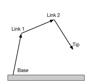
This 2D (planar) system is an example where it’s possible to over-constrain the end effector based on the system capabilities. Having more degrees of freedom certainly means more flexibility, and more of a chance to directly position and orient the end effector specifically as needed. The figure below shows that the flow is reversed from the Forward Kinematics. The tip position is known, and the pose of the arm is built to reach for or solve for the point in space. These points can be 1D, 2D or 3D, and even specify orientation.